Benjamin's Maths World

Installing and Importing the NumPy Package for Numerical Computing

Packages are organized collections of code for specific purpose(s). In this chapter, we will exclusively focus on the NumPy Python package, which specializes in efficient numerical computing and is essential for scientific applications. The first step is obviously to install and load the package. If the uv manager is used, then we can just recall the steps given in the very first tutorial. Afterwards, in order to use the package, we simply write an import statement: (import <package_name> as <alias>)

import numpy as np

We are then able to refer to functions (or anything else) in the NumPy package by utilizing the alias np.<function>.

Numpy Array

The most significant merit/selling point of the NumPy package is to enable the possibility to structure data/numbers into arrays according to given dimensions in a rectangular manner. (Imagine a matrix. We will see how it unfolds below very soon.) This provides several substantial advantages over the built-in list type. First, from a human perspective, arrays are easier to access and handle thanks to a convenient interface. Second, from a computer perspective, both the computational and storage efficiency are several orders of magnitude better, as the internal code for arrays has been optimized.

One-dimensional Array

To create a (one-dimensional) array from a list of data, we can simply use the np.array(<list>) definition:

x = np.array([1,2,3,-5,7,0])
y = np.array([2.5,-1.47,8,4.9])
print(x)
print(y)

which produces

[ 1  2  3 -5  7  0]
[ 2.5  -1.47  8.    4.9 ]

Notice how the outputs look different from the usual lists. We can index or slice an array just like how we deal with a list (see this tutorial). Using the same example:

print(x[3])
print(x[:-1:2])
print(y[0:2])

gives -5, [1 3 7], [ 2.5 -1.47] respectively. Assigning new values to components in an array also works similarly:

x[-2] = 4
y[1:] = 1.11, 2.22, 7.77
print(x)
print(y)

which now gives [ 1 2 3 -5 4 0] and [2.5 1.11 2.22 7.77]. An important caveat is that since we initialize x with all integer numbers, the array data type will also be fixed to be of integers. This causes the following problem if we write:

x[0] = 3.45
print(x)
print(x.dtype)

The dtype attribute stores the data type. This returns

[ 3  2  3 -5  7  0]
int64

This shows that the elements in that array are always cast to 64-bit integers (int64) even if we try to update them. This behavior can cause unexpected bugs and we should be wary of that.

Two important ways to generate arrays with fixed increment or spacing are np.arange(<start>, <end>, <step>) and np.linspace(<start>, <end>, <sample_num>). np.arange works just like the usual range but creates an array instead, and we will omit the explanation. It also does not include the end-point. Meanwhile, np.linspace generates an evenly spaced array with the number of sampling points indicated. For example,

x = np.linspace(-1,1,9)
print(x)

outputs [-1. -0.75 -0.5 -0.25 0. 0.25 0.5 0.75 1. ], a 9-point array.

Two-dimensional Arrays

Creation from Nested Lists

Meanwhile, to make two-dimensional (or higher-dimensional), rectangular arrays, the most fundamental way is to arrange the data into a nested list and use np.array again. For example,

X = np.array([[1, 2, -4, 5],
              [3, 0, -8, 7],
              [5, 9, -2, -1]])
print(X)

gives

[[ 1  2 -4  5]
 [ 3  0 -8  7]
 [ 5  9 -2 -1]]

Indexing for Multi-dimensional Arrays

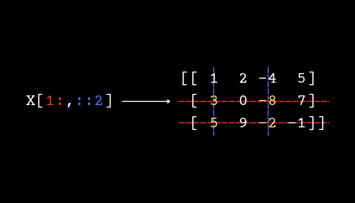
To reference element(s) inside a multi-dimensional array is a straightforward generalization of indexing where there are multiple dimensions and indices. Particularly, for two-dimensional arrays, we write something along the lines of <array>[row, column]. Using the above example, X[0,2] returns -4, X[1,3] returns 7, while X[-1,0] gives 5. Slicing also works similarly, dimension by dimension. Again, if we take the above example, if we write

print(X[1:,::2])
print(X[0,:])

we will obtain two subarrays (refer to the schematic below):

[[ 3 -8]
 [ 5 -2]]
[ 1  2 -4  5]

Other ways to make Multi-dimensional Arrays

There are numerous other approaches to make a two/multi-dimensional array from a group of smaller arrays. A direct way is to apply np.array again to compose a list of arrays. For instance,

a = np.array([1,4,5,3])
b = np.array([7,-2,1,0])
X = np.array([a,b])
print(X)

will output

[[ 1  4  5  3]
 [ 7 -2  1  0]]

They have been combined row by row. We can check the shape of this new array using the .shape method: print(X.shape) will produce (2, 4) (2 rows times 4 columns). An equivalent way is to use np.vstack (vertical stacking):

print(np.vstack([a,b]))

will also result in the same array as above. In contrast, we also have np.hstack (horizontal stacking):

print(np.hstack([a,b]))

that produces a one-dimensional array [ 1 4 5 3 7 -2 1 0] with \( 4 \times 2 = 8 \) components. In general, we may use the broader np.concatenate function to achieve both effects. If we write

print(np.concatenate([a,b]))

it will result in [ 1 4 5 3 7 -2 1 0] just like np.hstack. However, we may also do the following. First, we can enforce a and b to be explicit two-dimensional arrays with the shape (1,4) by the following syntax:

a2 = a[np.newaxis, :]
b2 = b[np.newaxis, :]

This adds an extra dummy dimension with np.newaxis. If we do print(a2) we will have [[1 4 5 3]] (notice the double square brackets). Then,

print(np.concatenate([a2, b2]))

will produce

[[ 1  4  5  3]
 [ 7 -2  1  0]]

again. If instead, we do

a2 = a[:, np.newaxis]
b2 = b[:, np.newaxis]
print(np.concatenate([a2, b2], axis=1))

we will have

[[ 1  7]
 [ 4 -2]
 [ 5  1]
 [ 3  0]]

because a2, b2 are now column vectors with the shape (4, 1), and then np.concatenate with the axis=1 parameter (default is 0, row by row) will concatenate the arrays along the second dimension (column by column).

Reshape

We can also create new arrays from existing ones by reshaping them. Unsurprisingly, we have the np.reshape(array, [shape]) function. Let’s just see the example below:

x = np.array([4,5,2,7,1,6,5,-3,0])
X = np.reshape(x, [3,3]) # or x.reshape([3,3])
print(X)

This will give

[[ 4  5  2]
 [ 7  1  6]
 [ 5 -3  0]]

so we have transformed the one-dimensional (9) array into a two-dimensional (3 times 3) one.

There is also the np.transpose function to swap axes. If we use this example, then

print(np.transpose(X, (1,0))) # Shorthand: X.T

will lead to the usual transpose in maths:

[[ 4  7  5]
 [ 5  1 -3]
 [ 2  6  0]]

Exercise

As a generalization, create a three-dimensional array (row, column, depth) with the shape (3,4,2) where at depth=0 it is

\begin{align}
\begin{bmatrix}
1 & 4 & 7 & 10 \\
2 & 5 & 8 & 11 \\
3 & 6 & 9 & 12
\end{bmatrix}
\end{align}

and at depth=1 it is

\begin{align}
\begin{bmatrix}
13 & 16 & 19 & 22 \\
14 & 17 & 20 & 23 \\
15 & 18 & 21 & 24
\end{bmatrix}
\end{align}

a1 = np.arange(1,3*4+1)
a2 = np.arange(3*4+1,3*4*2+1)

a1T = a1.reshape([4,3]).T
a2T = a2.reshape([4,3]).T

print(a1T, a2T)

print(np.concatenate([a1T[:,:,np.newaxis], a2T[:,:,np.newaxis]], axis=2))

[[[ 1 13]
  [ 4 16]
  [ 7 19]
  [10 22]]
 [[ 2 14]
  [ 5 17]
  [ 8 20]
  [11 23]]
 [[ 3 15]
  [ 6 18]
  [ 9 21]
  [12 24]]]

a1T = a1.reshape([3,4], order="F")
a2T = a2.reshape([3,4], order="F")

a = np.arange(3*4*2) + 1
print(a.reshape([3,4,2], order="F"))