Systems of First-order Linear ODEs in Matrix Form
Up until now, we have been focusing only on individual differential equations, one at a time. However, for many real-life problems, there are multiple ODEs, each of which is coupled to others in the system. This frequently happens in Earth System Science, where we have to consider the interactions between different variables, for instance, mass flows and chemical reactions between the reservoirs of various substances. This naturally leads to a system of ODEs. The simplest case would be that all of the ODEs involved are first-order, linear, having constant coefficients, and homogeneous. An \( n \times n \) system of such ODEs then takes the form of
\begin{align}
\left\{\begin{aligned}
\frac{dy_1}{dx} &= a_{11}y_1 + a_{12}y_2 + a_{13}y_3 + \cdots + a_{1n}y_n \\
\frac{dy_2}{dx} &= a_{21}y_1 + a_{22}y_2 + a_{23}y_3 + \cdots + a_{2n}y_n \\
\frac{dy_3}{dx} &= a_{31}y_1 + a_{32}y_2 + a_{33}y_3 + \cdots + a_{3n}y_n \\
&\vdots \\
\frac{dy_n}{dx} &= a_{n1}y_1 + a_{n2}y_2 + a_{n3}y_3 + \cdots + a_{nn}y_n \\
\end{aligned}\right. \tag{1}
\end{align}
where \( y_1, y_2, \ldots, y_n \) are the unknowns and \( a_{ij} \) are constants. We can compactly express this in matrix form:
\begin{equation}
\textbf{y}’ = A\textbf{y} \tag{2}
\end{equation}
where
\begin{align}
\textbf{y} &= \begin{bmatrix}
y_1 \\
y_2 \\
y_3 \\
\vdots \\
y_n
\end{bmatrix} & &
\textbf{y} = \begin{bmatrix}
\frac{dy_1}{dx} \\
\frac{dy_2}{dx} \\
\frac{dy_3}{dx} \\
\vdots \\
\frac{dy_n}{dx}
\end{bmatrix} \tag{3}
\end{align}
and
\begin{align}
A = \begin{bmatrix}
a_{11} & a_{12} & a_{13} & \cdots & a_{1n} \\
a_{21} & a_{22} & a_{23} & & a_{2n} \\
a_{31} & a_{32} & a_{33} & & a_{3n} \\
\vdots & & & \ddots & \vdots \\
a_{n1} & a_{n2} & a_{n3} & \cdots & a_{nn} \\
\end{bmatrix} \tag{4}
\end{align}
An example is the system
\begin{align}
\left\{\begin{aligned}
\frac{dy_1}{dx} &= 3y_1 -y_2 \\
\frac{dy_2}{dx} &= 2y_1 \end{aligned}\right. \tag{5}
\end{align}
which can be rewritten into
\begin{align}
\textbf{y}’ =
\begin{bmatrix} 3 & -1 \\
2 & 0 \end{bmatrix} \textbf{y} \tag{6}
\end{align}
Since each ODE concerning \( dy_i/dx \) for a fixed \( i \) now involves multiple dependent variables \( y_j \) on the R.H.S., we cannot use the usual method for solving a first-order linear ODE directly. However, we may make a change of variable such that \( \textbf{y} = P\textbf{z} \) and hence \( \textbf{y}’ = P\textbf{z}’ \). Then (2) becomes
\begin{align}
P\textbf{z}’ &= AP\textbf{z} \\
\textbf{z}’ &= P^{-1}AP \textbf{z} \tag{7}
\end{align}
According to Linear Algebra, \( P^{-1}AP \) is recognized as a similar matrix to \( P \). If we choose \( P \) such that its column fully consists of all distinct eigenvectors of \( A \), then it will be diagonalized into a diagonal matrix, such that \( P^{-1}AP = D \) with \( D \) only having non-zero entries, being the corresponding eigenvalues, along the main diagonal. When written out, the newly transformed ODEs become
\begin{align}
\left\{\begin{aligned}
\frac{dz_1}{dx} &= D_{11}z_1 \\
\frac{dz_2}{dx} &= D_{22}z_2 \\
\frac{dz_3}{dx} &= D_{33}z_3 \\
&\vdots \\
\frac{dz_n}{dx} &= D_{nn}z_n \\
\end{aligned}\right. \tag{8}
\end{align}
which are all solvable on their own, as each of them only involves a single dependent variable. From previous knowledge, the solutions will be \( z_j = c_je^{D_{jj}x} \). After working out \(z\) completely, we can recover the required solution in terms of the original variables simply by the inversion \( \textbf{y} = P\textbf{z} \).
Example
Now we will demonstrate by solving the following system of first-order ODEs:
\begin{align} \left\{\begin{aligned}
\frac{dy_1}{dx} &= 8y_1 -12y_2 + 14y_3 \\
\frac{dy_2}{dx} &= -2y_1 + 4y_2 -4y_3 \\
\frac{dy_3}{dx} &= -3y_1 + 6y_2 -5y_3
\end{aligned}\right. \tag{9}
\end{align}
where the initial conditions are \(y_1(0) = 3, y_2(0) = 1, y_3(0) = 5\).
The system written in matrix notation is
\begin{align}
\begin{bmatrix}
\frac{dy_1}{dx} \\
\frac{dy_2}{dx} \\
\frac{dy_3}{dx}
\end{bmatrix} =
\begin{bmatrix}
8 & -12 & 14 \\
-2 & 4 & -4 \\
-3 & 6 & -5
\end{bmatrix}
\begin{bmatrix}
y_1 \\
y_2 \\
y_3
\end{bmatrix} \tag{10}
\end{align}
The eigenvalues are calculated from
\begin{align}
\begin{vmatrix}
8-\lambda & -12 & 14 \\
-2 & 4-\lambda & -4 \\
-3 & 6 & -5-\lambda
\end{vmatrix} &= 0 \\
(1-\lambda)(2-\lambda)(4-\lambda) &= 0 \tag{11}
\end{align}
We will just show the steps for computing the eigenvector for \(\lambda = 1\) and leave the remaining to the readers. The Gaussian Elimination step is
\begin{align}
\left[\begin{array}{ccc|c}
7 & -12 & 14 & 0\\
-2 & 3 & -4 & 0 \\
-3 & 6 & -6 & 0
\end{array}\right] &\rightarrow
\left[\begin{array}{ccc|c}
1 & -2 & 2 & 0 \\
7 & -12 & 14 & 0 \\
-2 & 3 & -4 & 0 \\
\end{array}\right] & & \begin{aligned}R_3 \leftrightarrow R_1 \\
R_1/3 \rightarrow R_1
\end{aligned} \\
&\rightarrow
\left[\begin{array}{ccc|c}
1 & -2 & 2 & 0 \\
0 & 2 & 0 & 0 \\
0 & -1 & 0 & 0 \\
\end{array}\right] & & \begin{aligned}R_2 -7R_1 \rightarrow R_2 \\
R_3 + 2R_1 \rightarrow R_3
\end{aligned} \\
&\rightarrow
\left[\begin{array}{ccc|c}
1 & -2 & 2 & 0 \\
0 & 1 & 0 & 0 \\
0 & 0 & 0 & 0 \\
\end{array}\right] & & \begin{aligned}R_2/2 \rightarrow R_2 \\
R_3 + R_2 \rightarrow R_3
\end{aligned} \tag{12}
\end{align}
Hence the eigenvector for \( \lambda = 1 \) is \( (-2,0,1)^T \). It can be checked that the eigenvectors for \( \lambda = 2,4 \) are \( (-5,1,3)^T, (-4,1,2)^T \) respectively. Hence, by letting
\begin{equation}
P =
\begin{bmatrix}
-2 & -5 & -4 \\
0 & 1 & 1 \\
1 & 3 & 2
\end{bmatrix} \tag{13}
\end{equation}
then
\begin{align}
\textbf{y} &= P\textbf{z} \\
\begin{bmatrix}
y_1 \\
y_2 \\
y_3
\end{bmatrix} &=
\begin{bmatrix}
-2 & -5 & -4 \\
0 & 1 & 1 \\
1 & 3 & 2
\end{bmatrix}
\begin{bmatrix}
z_1 \\
z_2 \\
z_3
\end{bmatrix} \tag{14}
\end{align}
and the system is diagonalized as
\begin{align}
\begin{bmatrix}
\frac{dz_1}{dx} \\
\frac{dz_2}{dx} \\
\frac{dz_3}{dx}
\end{bmatrix}
&= \begin{bmatrix}
-2 & -5 & -4 \\
0 & 1 & 1 \\
1 & 3 & 2
\end{bmatrix}^{-1}
\begin{bmatrix}
8 & -12 & 14 \\
-2 & 4 & -4 \\
-3 & 6 & -5
\end{bmatrix}
\begin{bmatrix}
-2 & -5 & -4 \\
0 & 1 & 1 \\
1 & 3 & 2
\end{bmatrix} \\
&=
\begin{bmatrix}
1& 0 & 0 \\
0 & 2 & 0 \\
0 & 0 &4
\end{bmatrix}
\begin{bmatrix}
z_1 \\
z_2 \\
z_3
\end{bmatrix} \tag{15}
\end{align}
The solution for each of the components is then simply \(z_1 = c_1e^x, z_2 = c_2e^{2x}, z_3 = c_3e^{4x}\). The integration constants \(c_i\) can be determined by the initial conditions provided. Substituting them into the relation for change of variables gives
\begin{align}
\begin{bmatrix}
y_1(0) \\
y_2(0) \\
y_3(0) \end{bmatrix} &=
\begin{bmatrix}
-2 & -5 & -4 \\
0 & 1 & 1 \\
1 & 3 & 2 \end{bmatrix}
\begin{bmatrix}
z_1(0) \\
z_2(0) \\
z_3(0)
\end{bmatrix} \\
\begin{bmatrix}
3 \\
1 \\
5 \end{bmatrix} &=
\begin{bmatrix}
-2 & -5 & -4 \\
0 & 1 & 1 \\
1 & 3 & 2 \end{bmatrix}
\begin{bmatrix}
c_1 \\
c_2 \\
c_3 \end{bmatrix} \tag{16} \end{align}
It is not hard to obtain \(c_1 = -10, c_2 = 13, c_3 = -12\), and hence \(z_1 = -10e^x, z_2 = 13e^{2x}, z_3 = -12e^{4x}\). So the full solution for \(y_i\) is
\begin{align}
\begin{bmatrix}
y_1 \\
y_2 \\
y_3
\end{bmatrix}
&= \begin{bmatrix}
-2 & -5 & -4 \\
0 & 1 & 1 \\
1 & 3 & 2
\end{bmatrix}
\begin{bmatrix}
-10e^x \\
13e^{2x} \\
-12e^{4x}
\end{bmatrix} \\
\Rightarrow & \left\{\begin{aligned}
y_1 &= 20e^{x} -65e^{2x} + 48e^{4x} \\
y_2 &= 13e^{2x} -12e^{4x} \\
y_3 &= -10e^{x} + 39e^{2x} -24e^{4x}
\end{aligned}\right. \tag{17}
\end{align}
Equilibrium Points for Two-dimensional Linear Dynamical Systems
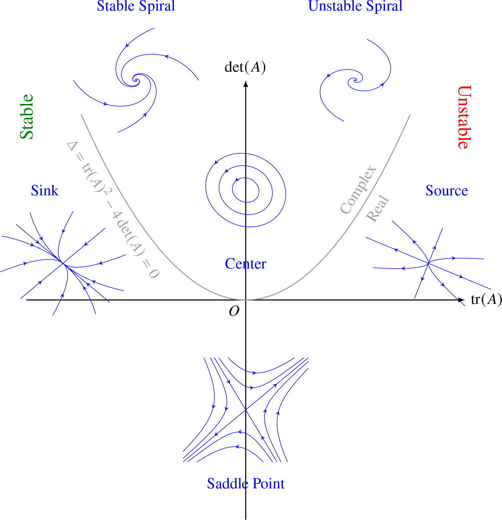
We will now concentrate on the particular case of two-dimensional dynamical systems \(\textbf{y}’ = A\textbf{y}\) where \(A\) is a real \(2 \times 2\) matrix. Their characteristics are then largely determined by the eigenvalues of \( A \) through diagonalization, as demonstrated above, assumed possible. Specifically, the solution trajectories/orbits will be described by \( z_1 = c_1e^{\lambda_1 t}, z_2 = c_2e^{\lambda_2 t} \) where \( \lambda_1, \lambda_2 \) are the two eigenvalues of \( A \), and \( z = (z_1, z_2)^T \) denotes the transformed coordinates in the eigenbasis. Accordingly, we can determine the types of equilibrium points at the origin, where \( \textbf{y}’ = A\textbf{0} = \textbf{0} \), and the behavior near them, based on the sign and magnitude of the two eigenvalues:

Notice that the trace and determinant of the matrix \( A \) will be invariants: \( \text{tr}(A) = \lambda_1 + \lambda_2, \det(A) = \lambda_1\lambda_2 \). These are exactly the sum and product of the roots for the characteristic polynomial, and by high school algebra we can readily infer the signs of the two eigenvalues from them. It can also be shown that the discriminant is equal to \( \text{tr}(A)^2 -4\det(A) \), thus we can deduce if the roots are real and distinct, real but repeated, or complex conjugates. Hence, we can infer the type of a given equilibrium point solely from the trace and determinant of \( A \). The classification and the corresponding phase portraits are visualized in the schematic as follows.

Exercise
A chemical tracer \(P\) decays into another tracer \(Q\), which in turn decays to produce yet another tracer \(R\). Both reactions are first-order:
\begin{align}
P \xrightarrow{k_1} Q \xrightarrow{k_2} R \tag{18}
\end{align}
and hence have rate laws in the form of
\begin{align}
\left\{\begin{aligned}
\frac{d[P]}{dt} &= -k_1[P] \\
\frac{d[Q]}{dt} &= k_1[P] -k_2[Q] \\
\frac{d[R]}{dt} &= k_2[Q]
\end{aligned} \right. \tag{19}
\end{align}
Initially, \([P] = 1\) mol per unit volume and \([Q] = [R] = 0\). (\(k_1, k_2\) have the unit of \(\text{s}^{-1}\)). Express the time evolution of concentrations for all the three tracers \([P], [Q], [R]\), and find the time \(t_Q\) where \([Q]\) reaches its maximum in terms of \(k_1, k_2\).
Answer
The three ODEs can be written as a matrix system of
\begin{align}
\textbf{y}’ = A\textbf{y} =
\begin{bmatrix}
-k_1 & 0 & 0 \\
k_1 & -k_2 & 0 \\
0 & k_2 & 0
\end{bmatrix} \textbf{y}
\end{align}
It is easy to see that the eigenvalues of the lower-triangular coefficient matrix \(A\) are \(0\), \(-k_1\), and \(-k_2\). We further assume that \(k_1 \neq k_2\). The eigenvector for \(\lambda = 0\) is clearly \((0,0,1)^T\), while that for \(\lambda = -k_1\) can be derived from solving
\begin{align}
\left[\begin{array}{ccc|c}
0 & 0 & 0 & 0 \\
k_1 & k_1-k_2 & 0 & 0 \\
0 & k_2 & k_1 & 0 \\
\end{array}\right]
\end{align}
which leads to an eigenvector of \((k_1-k_2,-k_1,k_2)^T\). Similarly, the eigenvector for \(\lambda = -k_2\) can be checked to be \((0,-1,1)^T\). The matrix for change of variables will then be
\begin{align}
P = \begin{bmatrix}
k_1-k_2 & 0 & 0 \\
-k_1 & -1 & 0 \\
k_2 & 1 & 1
\end{bmatrix}
\end{align}
and with \(\textbf{y} = P\textbf{z}\) we have
\begin{align}
\textbf{z}’ &= (P^{-1}AP)\textbf{z} = D\textbf{z}\\
&=
\begin{bmatrix}
-k_1 & 0 & 0 \\
0 & -k_2 & 0 \\
0 & 0 & 0 \end{bmatrix}\textbf{z}
\end{align}
the solution of which is \(z_1 = c_1e^{-k_1t}, z_2 = c_2e^{-k_2t}, z_3 = c_3\). The initial conditions of \([P] = 1, [Q] = [R] = 0\) mean that
\begin{align}
\textbf{y}(0) &= P\textbf{z}(0) \\
\begin{bmatrix} 1 \\ 0 \\ 0 \end{bmatrix}
&= \begin{bmatrix}
k_1-k_2 & 0 & 0\\
-k_1 & -1 & 0 \\
k_2 & 1 & 1 \end{bmatrix}
\begin{bmatrix} c_1 \\ c_2 \\ c_3 \end{bmatrix} \end{align}
Solving for it yields \(c_1 = \frac{1}{k_1-k_2}, c_2 = -\frac{k_1}{k_1-k_2}, c_3 = 1\). Therefore, \(z_1 = \frac{1}{k_1-k_2}e^{-k_1t}, z_2 = -\frac{k_1}{k_1-k_2}e^{-k_2t}, z_3 = 1\), and
\begin{align}
\textbf{y} &= \begin{bmatrix}
k_1-k_2 & 0 & 0\\
-k_1 & -1 & 0\\
k_2 & 1 & 1 \end{bmatrix}
\begin{bmatrix}
\frac{1}{k_1-k_2}e^{-k_1t} \\
-\frac{k_1}{k_1-k_2}e^{-k_2t} \\
1 \end{bmatrix} \\
&= \begin{bmatrix}
e^{-k_1t} \\
-\frac{k_1}{k_1-k_2}e^{-k_1t} + \frac{k_1}{k_1-k_2}e^{-k_2t} \\
\frac{k_2}{k_1-k_2}e^{-k_1t} -\frac{k_1}{k_1-k_2}e^{-k_2t} + 1 \end{bmatrix}
\end{align}
Hence
\begin{align}
[P] &= e^{-k_1t} \\
[Q] &= -\frac{k_1}{k_1-k_2}e^{-k_1t} + \frac{k_1}{k_1-k_2}e^{-k_2t} \\
[R] &= \frac{k_2}{k_1-k_2}e^{-k_1t} -\frac{k_1}{k_1-k_2}e^{-k_2t} + 1
\end{align}
The time \(t_Q\) where \([Q]\) reaches maximum occurs when \(\frac{d[Q]}{dt} = 0\), which leads to
\begin{align}
\frac{d[Q]}{dt} = k_1[P] -k_2[Q] &= 0 \\
k_1e^{-k_1 t} -k_2(-\frac{k_1}{(k_1-k_2)}e^{-k_1 t} + \frac{k_1}{(k_1-k_2)}e^{-k_2t}) &= 0 \\
k_1e^{-k_1 t} + \frac{k_1k_2}{(k_1-k_2)}e^{-k_1 t} -\frac{k_1k_2}{(k_1-k_2)}e^{-k_2t} &= 0 \\ \frac{k_1^2}{(k_1-k_2)}e^{-k_1 t} -\frac{k_1k_2}{(k_1-k_2)}e^{-k_2t} &= 0 \\
\frac{k_1^2}{(k_1-k_2)}e^{-k_1 t} &= \frac{k_1k_2}{(k_1-k_2)}e^{-k_2t} \\
e^{-(k_1-k_2)t} &= \frac{k_2}{k_1} \\
-(k_1-k_2)t &= \ln\left(\frac{k_2}{k_1}\right) \\
\Rightarrow t_Q = -\frac{\ln(\frac{k_2}{k_1})}{k_1 -k_2} &= \frac{\ln k_1 -\ln k_2}{k_1 -k_2} \end{align}



Leave a Reply