Solving the Laplace equation in spherical coordinates
Now, we will discuss the last case of setup for the Laplace equation, a three-dimensional space with spherical coordinates. The Laplacian in spherical coordinates is
\begin{align}
\nabla^2 = \frac{1}{r^2} \frac{\partial}{\partial r} (r^2\frac{\partial}{\partial r}) + \frac{1}{r^2\sin^2 \phi}\frac{\partial^2}{\partial \theta^2} + \frac{1}{r^2\sin \phi} \frac{\partial}{\partial \phi} (\sin\phi \frac{\partial}{\partial \phi}) \tag{1}
\end{align}
where \(r\) is the radius, \( \theta \) is the azimuthal angle, \( \phi \) is the zenith angle. The corresponding Laplace equation then reads
\begin{align}
\nabla^2 u (r,\theta,\phi) = \frac{1}{r^2} \frac{\partial}{\partial r} (r^2\frac{\partial u}{\partial r}) + \frac{1}{r^2\sin^2 \phi}\frac{\partial^2 u}{\partial \theta^2} + \frac{1}{r^2\sin \phi} \frac{\partial}{\partial \phi} (\sin\phi \frac{\partial u}{\partial \phi}) = 0 \tag{2}
\end{align}
Just like before, we employ the method of Separation of Variables. Here we let
\begin{align}
u(r,\theta,\phi) = R(r)\Theta(\theta)\Phi(\phi) \tag{3}
\end{align}
Substituting this into (2), we have
\begin{align}
\frac{1}{r^2} \frac{\partial}{\partial r} (r^2R’\Theta\Phi) + \frac{1}{r^2\sin^2 \phi}R\Theta^{\prime\prime}\Phi + \frac{1}{r^2\sin \phi} \frac{\partial}{\partial \phi} ((\sin\phi) R\Theta\Phi’) &= 0 \\
\frac{1}{R} \frac{\partial}{\partial r} (r^2R’) + \frac{1}{\sin^2 \phi}\frac{\Theta^{\prime\prime}}{\Theta} + \frac{1}{(\sin \phi)\Phi} \frac{\partial}{\partial \phi} ((\sin\phi) \Phi’) &= 0 \tag{4}
\end{align}
where we have divided by \( R\Theta\Phi \) and multiply by \(r^2\). The first term only depends on \( r \) while the last two terms depend on \(\theta\) and \(\phi\). Hence we can write
\begin{align}
\frac{1}{R} \frac{\partial}{\partial r} (r^2R’) &= \lambda \tag{5} \\
\frac{1}{\sin^2 \phi}\frac{\Theta^{\prime\prime}}{\Theta} + \frac{1}{(\sin \phi)\Phi} \frac{\partial}{\partial \phi} ((\sin\phi) \Phi’) &= -\lambda \tag{6}
\end{align}
(5) can be further cast into
\begin{align}
r^2R^{\prime\prime} + 2rR’ &= \lambda R \\
r^2R^{\prime\prime} + 2rR’ -\lambda R &= 0 \tag{7}
\end{align}
This is an Euler form ODE (see this tutorial), with the general solution of
\begin{align}
R = Ar^{p_1} + Br^{p_2} \tag{8}
\end{align}
where the corresponding auxiliary equation requires that
\begin{align}
p^2 + (2-1)p -\lambda &= 0 \\
p^2 + p -\lambda &= 0 \tag{9}
\end{align}
and thus \( p_1 + p_2 = -1 \), \( p_1p_2 = -\lambda \). So we can let \( p_1 = l \), \( p_2 = -(l+1) \), where now \(\lambda = l(l+1)\). Now, we proceed to further separate (6). By multiplying \( \sin^2 \phi \), we have
\begin{align}
\frac{\Theta^{\prime\prime}}{\Theta} + \frac{\sin \phi}{\Phi} \frac{\partial}{\partial \phi} ((\sin\phi) \Phi’) &= -l(l+1) \sin^2 \phi \\
\frac{\Theta^{\prime\prime}}{\Theta} + \frac{\sin \phi}{\Phi} \frac{\partial}{\partial \phi} ((\sin\phi) \Phi’) + l(l+1) \sin^2 \phi &= 0 \tag{10}
\end{align}
Since the first term depends on \(\theta\) only while the subsequent terms depend on \( \phi \) only, we may take
\begin{align}
\frac{\Theta^{\prime\prime}}{\Theta} &= -m^2 \tag{11} \\
\frac{\sin \phi}{\Phi} \frac{\partial}{\partial \phi} ((\sin\phi) \Phi’) + l(l+1) \sin^2 \phi &= m^2 \tag{12}
\end{align}
(11) has the familiar Fourier solution:
\begin{align}
\Theta^{\prime\prime} + m^2\Theta &= 0 \\
\Theta &= C \cos (m\theta) + D\sin(m\theta) \tag{13}
\end{align}
Just like the cylindrical case, we require \( m = 0,1,2,\ldots \) to be an integer for single-valuedness. The final step is to deal with (12). The trick is to make a change of variable \( x = \cos\phi \), then \( dx/d\phi = -\sin\phi \) and \( d/d\phi = -(\sin\phi) d/dx = -\sqrt{1-x^2} d/dx \). (12) then becomes
\begin{align}
\sin \phi \frac{d}{d\phi} ((\sin\phi) \frac{d\Phi}{d\phi}) + l(l+1) (\sin^2 \phi) \Phi &= m^2 \Phi \\
-\sin^2 \phi \frac{d}{dx} (-(\sin\phi)^2 \frac{d\Phi}{dx}) + l(l+1) (\sin^2 \phi) \Phi -m^2 \Phi &= 0 \\
\frac{d}{dx} ((1-x^2) \frac{d\Phi}{dx}) + (l(l+1) -\frac{m^2}{1-x^2}) \Phi &= 0 \tag{14}
\end{align}
This equation is known as the associated Legendre equation. Compared with the original Legendre equation (see (8) in this tutorial), the only difference is the addition of the \( -\frac{m^2}{1-x^2} \) part. The corresponding solutions, the associated Legendre functions, will be controlled by the parameters \(l\) and \(m\):
\begin{align}
\Phi = EP_{l}^m(x) + FQ_{l}^m(x) \tag{15}
\end{align}
Therefore, the most general solution for the Laplace equation will look like
\begin{align}
u(r,\theta,\phi) = (Ar^{l} + Br^{-(l+1)})(C \cos (m\theta) + D\sin(m\theta))(EP_{l}^m(\cos\phi) + FQ_{l}^m(\cos\phi)) \tag{16}
\end{align}
We will not go into the details about the associated Legendre functions but only state those properties that are necessary for our next argument. They can be given by the Rodrigues’ formula when \(l, m\) are integers:
\begin{align}
P_{l}^m(x) &= (1-x^2)^{|m|/2} \frac{d^{|m|}}{dx^{|m|}} (P_l(x)) \tag{17}
\end{align}
where \( P_l \) is the original Legendre function of the first kind. The formula is similar for \( Q_{l}^m \). In fact, in order to ensure that the zenith part of the solution (15) is finite at the poles (when \(\phi = 0, \pi\) and \(x = \cos\phi = \pm 1\)), we will set \(F\) to zero and demand that \( l \) be an integer as well since \( Q_l^m \) will always diverge at \( x = \pm 1\), and so do \( P_l^m\) if \(l\) is not an integer. Note that we also require \( |m| \leq l \) as \( P_l^m = 0\) if \( m > l \) as seen from (17). If \( m = 0\), then the associated Legendre equation/functions will just reduce to the old one. Moreover, if the domain includes the origin \( r = 0 \), then we also need to take \( B = 0 \) to avoid singularity.
So, under the finiteness condition, the azimuthal and zenith parts in (16), when combined, are
\begin{align}
\Theta(\theta)\Phi(\phi) = P_{l}^m(\cos\phi)(C \cos (m\theta) + D\sin(m\theta)) \tag{18}
\end{align}
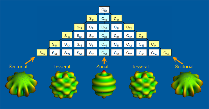
This form frequently arises in many physical and geoscience applications, and bears the special name of spherical harmonics. They are defined with a normalization factor, as
\begin{align}
Y_l^m(\theta,\phi) = (-1)^m(\frac{2l+1}{4\pi}\frac{(l-m)!}{(l+m)!})^{1/2} P_l^m(\cos\phi) e^{im\theta} \tag{19}
\end{align}
Thus the physical solution of the Laplace equation may be compactly written as just
\begin{align}
u(r,\theta,\phi) = (Ar^{l} + Br^{-(l+1)})Y_l^m(\theta,\phi) \tag{20}
\end{align}
Example
A homogeneous solid ball of radius \(a\) is kept at a temperature \( T_0 \) on the surface of its northern hemisphere and \( -T_0 \) on its southern hemisphere surface. Find the equilibrium temperature of the ball.
The corresponding boundary condition is
\begin{align}
u(a,\theta,\phi) = \begin{cases}
T_0 & & 0 \leq \phi < \pi/2, 0 < \cos\phi \leq 1 \\
-T_0 & & \pi/2 < \phi \leq \pi, -1 \leq \cos\phi < 0 \\
\end{cases} \tag{21}
\end{align}
The axial symmetry of this problem means that there will be no \( \theta \) dependence and hence \( m = 0 \). Moreover, to have a physical solution, \( B = F = 0 \) in (16) as it has to be finite at both the center and north/south poles. Hence the form of the solution will be
\begin{align}
u(r,\theta,\phi) = \sum_{l=0}^{\infty} A_lr^{l}P_{l}(\cos\phi) \tag{22}
\end{align}
To match the B.C., we need
\begin{align}
u(a,\theta,\phi) = \sum_{l=0}^{\infty} A_la^{l}P_{l}(\cos\phi) \tag{23}
\end{align}
By the orthogonality of the Legendre polynomials, we have, with \( x = \cos\phi \):
\begin{align}
A_la^{l} &= \frac{2l+1}{2} \int_{-1}^{1} u(a,\theta,\phi)P_{l}(x) dx \\
&= \frac{2l+1}{2} T_0 (\int_{0}^{1} P_{l}(x) dx -\int_{-1}^{0} P_{l}(x) dx) \tag{24}
\end{align}
Further exploiting the odd/even symmetry of the Legendre polynomials, we have
\begin{align}
A_{2k} &= 0 \tag{25} \\
A_{2k+1}a^{2k+1} &= (4k+3) T_0 \int_{0}^{1} P_{2k+1}(x) dx \tag{26}
\end{align}
We state the first few values of integrals for even-order Legendre polynomials below.
\begin{align}
\begin{aligned}
\int_{0}^{1} P_{1}(x) dx &= \frac{1}{2} \\
\int_{0}^{1} P_{3}(x) dx &= -\frac{1}{8} \\
\int_{0}^{1} P_{5}(x) dx &= \frac{1}{16}
\end{aligned} \tag{27}
\end{align}
And so our desired solution will be
\begin{align}
u = T_0(\frac{3}{2}(\frac{r}{a})P_{1}(\cos\phi) -\frac{7}{8}(\frac{r}{a})^3 P_{3}(\cos\phi) + \frac{11}{16}(\frac{r}{a})^5 P_{5}(\cos\phi) -\cdots) \tag{28}
\end{align}
Exercise
The gravitational potential of the Earth also follows the Laplace equation. If we make a simplification and treat our Earth as a homogeneous ellipsoid, which terms of the solution (16)/(20) remain?
Answer
Since the gravity of the Earth is exerted outside itself, in (16) we have \( A = 0 \) instead, so that the gravitational potential at the far field diminishes. The north-south symmetry requires that \( l = 2p \) to be even. Assume that the line \( \theta = 0, \pi \) aligns with one of the axes of the ellipsoid, then the ellipsoidal equatorial plane means that in (16), \(D = 0\) while \( C \) only has a non-zero value when \( m = 2q \) is also even. So the general solution for the simplified Earth’s gravitational potential will be
\begin{align}
V = \frac{GM}{r} (1 + \sum_{p=1}^{\infty}\sum_{q=0}^p (\frac{R}{r})^{2p} C_{2p,2q} \cos (2q\theta) P_{2p}^{2q}(\cos\phi))
\end{align}
where \( GM/r \) is the asymptotic expression of the Earth’s gravitational potential at a large distance.

(Schematic taken from Ince et al. (2019): ICGEM – 15 years of successful collection and distribution of global gravitational models, associated services, and future plans)


Leave a Reply