Definition and Motivation of Convolution
Convolution is carried out for two functions \( f(x), g(x) \), defined as
\begin{align}
[f*g](x) = \int_{-\infty}^{\infty} f(u)g(x-u) du \tag{1}
\end{align}
To understand why the form of convolution is like this, we can imagine \(f(x)\) is the distribution of mass/signal (e.g. electric charge, sea surface temperature), while \( g(x) \) is the physical response to a unit amount of the signal (impulse) (e.g. electric field due to an electric charge, atmospheric convection due to SST heating). The convolution \( [f*g](x) \) is subsequently the overall large-scale physical pattern arising from all the masses/signals combined (e.g. the net resulting electric field/atmospheric flow throughout the space). At a fixed location \(x\), it will consist of all the responses, due to some impulse at \( u \) and the reaction to it at a displacement of \( x -u \) away (\( u + (x-u) = x \)).

Notice that convolution is symmetric so that we can exchange the roles of \( f \) and \( g \) as we see fit:
\begin{align}
[f*g](x) &= \int_{u=-\infty}^{u=\infty} f(u)g(x-u) du \\
&= \int_{v=\infty}^{v=-\infty} f(x-v)g(v) d(x-v) && (v = x-u) \\
&= -\int_{\infty}^{-\infty} f(x-v)g(v) dv \\
&= \int_{-\infty}^{\infty} f(x-v)g(v) dv \tag{2}
\end{align}
(\(u\) and \(v\) are just dummy variables) The major result about convolution in the context of Laplace Transform is the Convolution Theorem. Notice that, since for the Laplace Transform, the input functions are confined to \( x > 0 \), the lower[upper] limit of (1) or (2) will be truncated to \(0\) [\(x\)], i.e.
\begin{align}
[f*g](x) = \int_{0}^{x} f(u)g(x-u) du = \int_{0}^{x} f(x-v)g(v) dv \tag{3}
\end{align}
then we can start proving the desired theorem:
\begin{align}
\mathcal{L}[f*g](s) &= F(s)G(s) \tag{4}
\end{align}
i.e. the Laplace Transform of a convolution is simply the product of the respective Laplace Transforms \( F, G \) of the two involved functions \( f,g \). Starting from the R.H.S. (using time as the physical variable for now), we have
\begin{align}
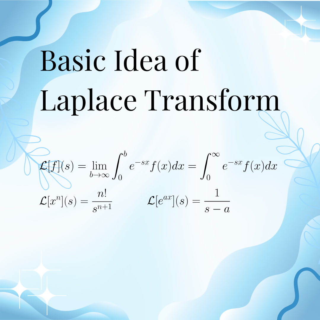
F(s)G(s) &= (\int_0^{\infty} e^{-s\tau’} f(\tau’) d\tau’) (\int_0^{\infty} e^{-s\tau} g(\tau) d\tau) \\
&= \int_0^{\infty} \int_0^{\infty} e^{-s(\tau’+\tau)} f(\tau’) g(\tau) d\tau’ d\tau \\
&= \int_0^{\infty} (\int_0^{\infty} e^{-s(\tau’+\tau)} f(\tau’) d\tau’) g(\tau) d\tau \tag{5}
\end{align}
Let \( \tau’+\tau = t \), so that \( \tau’ = t-\tau\) (where \(\tau\) is fixed during integration in the inner integral) and \(d\tau’ = dt\), hence
\begin{align}
&\quad \int_0^{\infty} (\int_0^{\infty} e^{-s(\tau’+\tau)} f(\tau’) d\tau’) g(\tau) d\tau \\
&= \int_0^{\infty} (\int_{\tau}^{\infty} e^{-st} f(t-\tau) dt) g(\tau) d\tau \\
&= \int_0^{\infty} \int_{\tau}^{\infty} e^{-st} f(t-\tau) g(\tau) dt d\tau \tag{6}
\end{align}
According to the schematic below, we can switch the order of integration as
\begin{align}
&\quad \int_{\tau=0}^{\tau=\infty} \int_{t=\tau}^{t=\infty} e^{-st} f(t-\tau) g(\tau) dt d\tau \\
&= \int_{t=0}^{t=\infty} \int_{\tau=0}^{\tau=t} e^{-st} f(t-\tau) g(\tau) d\tau dt \\
&= \int_{t=0}^{t=\infty} e^{-st} (\int_{\tau=0}^{\tau=t} f(t-\tau) g(\tau) d\tau) dt \\
&= \int_{t=0}^{t=\infty} e^{-st} (f(t) * g(t)) dt = \mathcal{L}[f*g](s) \tag{7}
\end{align}
and so (4) is proved.

Laplace Transform of an Integral
By the Convolution Theorem, we can swiftly derive the Laplace Transform of an integral in general: putting \( g = 1 \) in (3) and applying (4) gives
\begin{align}
\mathcal{L}[\int_0^t f(\tau) d\tau](s) = \mathcal{L}[f*g](s) = F(s)G(s) = \frac{F(s)}{s} \tag{8}
\end{align}
by recalling that the Laplace transform of \( 1 \) is just \( 1/s \).
Exercise
Find the Inverse Laplace Transform of
\begin{align}
\frac{s}{(s^2+1)^2} = (\frac{1}{s^2+1})(\frac{s}{s^2+1}) \tag{9}
\end{align}
by Convolution Theorem. Hence deduce the Laplace Transform of \(t \sin t\).
Answer
The two factors on the R.H.S. are obviously the Laplace Transforms for \(\sin(t)\) and \(\cos(t)\). By (4), its inverse is
\begin{align}
&\quad \int_0^t \sin(\tau) \cos(t-\tau) d\tau \\
&= \int_0^t \frac{1}{2} [\sin(\tau + (t-\tau)) + \sin(\tau -(t-\tau))] d\tau \\
&= \frac{1}{2} \int_0^t (\sin t + \sin(2\tau -t)) d\tau \\
&= \frac{1}{2} [\tau \sin t -\frac{1}{2}\cos(2\tau -t)]_0^t \\
&= \frac{1}{2} (t\sin t + 0) = \frac{1}{2} t\sin t
\end{align}
where at the start we have used the product-to-sum trigonometric formula. Hence
\begin{align}
\mathcal{L}[\frac{1}{2} t\sin t] &= \frac{s}{(s^2+1)^2} \\
\mathcal{L}[t\sin t] &= \frac{2s}{(s^2+1)^2}
\end{align}


Leave a Reply