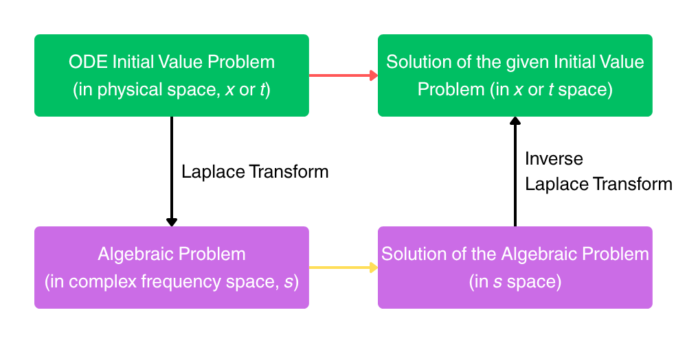
Heaviside Step Function and Dirac Delta Function
Before getting into using Laplace Transform to solve ODEs, we shall study two special kinds of functions that frequently show up in such a context. The first one is the Heaviside Step Function, which, as its name suggests, appears as a flat unit rise to the right like a step (see the graph below). The definition of the step function is naturally
\begin{align}
H(x) =
\begin{cases}
1 & \text{when } x > 0 \\
0 & \text{when } x < 0
\end{cases} \tag{1}
\end{align}
(the exact value at \(x = 0\) depends on the scenario, usually it will be \(1/2\) if defined.)

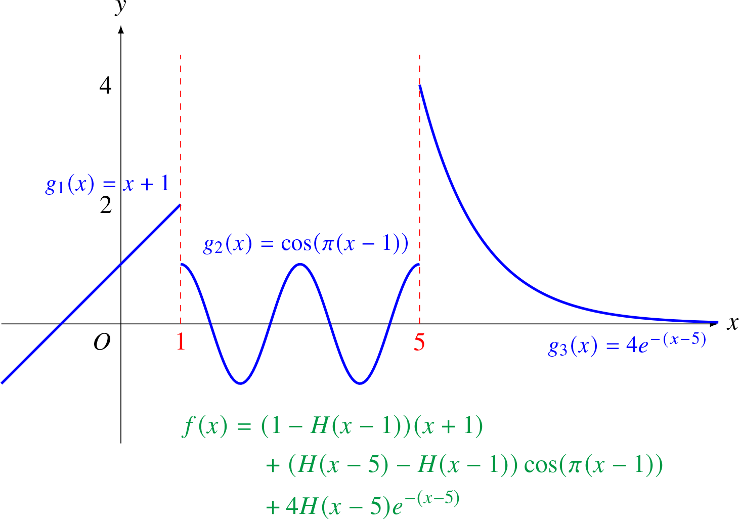
Subsequently, the step function \( H(x-a) \) (shifted by \(a\)) is then like a switch that turns on after \(x = a\). For example, the value of \(3xH(x-2)\) remains \(0\) for \(x < 2\), but becomes just \(3x\) for \(x > 2\). In this case, at \(x = 2\), \(xH(x-2)\) is discontinuous where the left limit is \(0\) but the right limit is \(3(2) = 6\). To generalize, we can use the step function to define a piecewise continuous function, formed by gluing different pieces of functions that are themselves continuous, end-to-end at finitely many points. If at such a point it is discontinuous, then at least it should have a finite left limit when approaching from the left, and similarly a finite right limit, although they may not be equal. Mathematically, if
\begin{align}
f(x) =
\begin{cases}
g_1(x) & x > x_1 \\
g_2(x) & x_1 < x < x_2 \\
g_3(x) & x_2 < x < x_3 \\
\vdots & \\
g_n(x) & x_{n-1} < x < x_n \\
\vdots &
\end{cases} \tag{2}
\end{align}
(provided all the \(g_n(x)\) are continuous over each corresponding interval) then we can rewrite it using the Heaviside step functions as
\begin{align}
f(x) &= \begin{aligned} &(1-H(x-x_1))g_1(x) + (H(x-x_1)-H(x-x_2))g_2(x) \\
&+ \cdots + (H(x-x_{n-1})-H(x-x_n))g_n(x) + \cdots \end{aligned} \tag{3} \\
&= \begin{aligned} &g_1(x) + H(x-x_1)(g_2(x) -g_1(x)) + \cdots \\
&+ H(x-x_{n-1})(g_n(x) -g_{n-1}(x)) + \cdots \end{aligned} \tag{4}
\end{align}
in two ways. Below shows an example of a piecewise continuous function that consists of three smaller functions.

The Laplace Transform of the step function centered at \(x = a\) is then by definition ((1) of the last tutorial):
\begin{align}
\mathcal{L}[H(x-a)](s) &= \int_0^{\infty} e^{-sx} H(x-a) dx \\
&= \int_0^{a} e^{-sx} H(x-a) dx + \int_a^{\infty} e^{-sx} H(x-a) dx \\
&= \int_0^{a} e^{-sx} (0) dx + \int_a^{\infty} e^{-sx} (1) dx \\
&= 0 + [-\frac{1}{s}e^{-sx}]_a^{\infty} \\
&= \frac{e^{-sa}}{s} \tag{5}
\end{align}
where we have applied (1) over the two split integration intervals respectively.
Another interesting function is the Dirac Delta Function. It is often described to be
\begin{align}
\delta(x) =
\begin{cases}
\infty & \text{when } x = 0 \\
0 & \text{else } x \neq 0
\end{cases} \tag{6}
\end{align}
and having the property of
\begin{align}
\int_{-\infty}^{\infty} \delta(x) f(x) dx = f(0) \tag{7}
\end{align}
While (6) is not a really rigorous way to define the delta function, (7) is a better definition that characterizes it. From (7), we can easily derive two more results: by taking \( f(x) = 1 \),
\begin{align}
\int_{-\infty}^{\infty} \delta(x) dx = 1 \tag{8}
\end{align}
and make a change of variable \( x \to x-a \):
\begin{align}
\int_{-\infty}^{\infty} \delta(x-a) f(x-a) d(x-a) &= f(x-a=0) \\
\int_{-\infty}^{\infty} \delta(x-a) f(x-a) dx &= f(a) \tag{9}
\end{align}
From (6) and (8), we can visualize that the delta function is physically a unit pulse/signal over an infinitesimally small time window. It can be thought of a rectangle that has a width of \( \epsilon \) and a height of \(1/\epsilon\), where \( \epsilon \to 0 \). Meanwhile, (9) implies that the role of the delta function \( \delta(x-a)\) in an integral is to extract the value of \(f(x)\) at a fixed point \(x = a\) (the integration interval can be any that includes this point), hence sometimes the delta function is also called the sampling function in areas like signal processing. (see the schematic below)

The Laplace Transform of the delta function located at \(x = a\) is thus by definition (again (1) of the last tutorial and (9) just above):
\begin{align}
\mathcal{L}[\delta(x-a)](s) &= \int_0^{\infty} e^{-sx} \delta(x-a) dx \\
&= e^{-sa} \tag{10}
\end{align}
First and Second Shifting Theorems
There are two shifting theorems for the Laplace Transform. Let’s denote the Laplace Transform of \( f(x) \) as \( F(s) \). The first shifting theorem is relatively easy to get:
\begin{align}
\mathcal{L}[e^{ax}f](s) &= \int_0^{\infty} e^{-sx} e^{ax} f(x) dx \\
&= \int_0^{\infty} e^{-(s-a)x} f(x) dx \\
&= F(s-a) \tag{11}
\end{align}
and the second shifting theorem considers translating the original function \( f(x), x > 0 \) to the right, truncated to the left by the Heaviside step function:
\begin{align}
&\quad \mathcal{L}[H(x-a)f(x-a)](s) \\
&= \int_0^{\infty} e^{-sx}H(x-a)f(x-a) dx \\
&= \int_a^{\infty} e^{-sx}f(x-a) dx && \text{(by (1))}\\
&= \int_0^{\infty} e^{-s(x+a)}f(x) d(x+a) && \text{(\(x \to x+a\))}\\
&= e^{-sa} \int_0^{\infty} e^{-sx}f(x) dx = e^{-sa}F(s) \tag{12}
\end{align}
The interpretations for these two theorems are as follows. For (12), if we want to shift a function over the physical space, then we have to multiply by \( e^{-sa} \) in the complex frequency domain. On the other hand, regarding (11), if we would like to shift a function in the complex space, then we ought to multiply the physical function by \(e^{ax}\). These combined are essentially a duality between the two spaces.
Derivative/Integral of Laplace Transform
Finally, we will show what happens if we differentiate a given Laplace Transform. By Leibniz Integral Rule, we may differentiate under the integral sign to obtain
\begin{align}
\frac{d}{ds}F(s) &= \frac{d}{ds} \int_0^{\infty} e^{-sx}f(x) dx \\
F'(s) &= \int_0^{\infty} \frac{\partial}{\partial s}(e^{-sx}f(x)) dx \\
&= \int_0^{\infty} -te^{-sx}f(x) dx \\
&= \mathcal{L}[-tf(x)](s) \tag{13}
\end{align}
which means that the inverse transform of a derivative in the complex domain corresponds to the original physical function times \(-t\). Extending (13) in the opposite direction, we can also inquire about the result of integrating a Laplace transform:
\begin{align}
-\frac{d}{ds} \int_s^{\infty} F(s) ds = F(s) &= \mathcal{L}[f(x)](s) = -\mathcal{L}[-\frac{tf(x)}{t}](s) \\
\int_s^{\infty} F(s) ds &= \mathcal{L}[\frac{f(x)}{t}](s) \tag{14}
\end{align}
(It is not hard to show that for the integration constant to be consistent, the upper limit of the integral must be \( \infty \).)
Exercise
Find the Laplace Transforms of the following functions:
- \(3e^{2t}t^2\)
- \(e^t\cos(4t)\)
- \( tH(t-2) \)
and the inverse Laplace Transforms of:
- \( 5/(s+1)^2 + 1/(s-3) \)
- \( 2/(s^2-2s+3) \) (Hint: Completing square)
- \( e^{-s}/(s+2)^3 \)
Answer
For the first part,
- By (11), the Laplace Transform will be shifted by \(2\) to become \( 6/(s-2)^3 \).
- Again by (11), it will be \( (s-1)/((s-1)^2+4^2) = (s-1)/(s^2-2s+17) \).
- For (12), \( a = 2 \) and \( t = (t-2)+2 \), so the Laplace Transform should be \( e^{-2s} (1/s^2 + 2/s) \). (can also via (13))
For the second part,
- With (11), the inverse Laplace Transform is \( 5te^{-t} + e^{3t} \).
- Note that \(2/(s^2-2s+3) = 2/((s-1)^2+(\sqrt{2})^2) \), so the required inverse is \( \sqrt{2} \sin(\sqrt{2}t) e^t \).
- By both (11) and (12), the inverse Laplace Transform will be \(H(t-1)e^{-2(t-1)}(t-1)^2/2 \).


Leave a Reply