Benjamin's Maths World

Expanding Functions using Legendre Polynomials

Since the Legendre Equation is a Sturm-Liouville Equation, by the Spectral Theorem (see this tutorial), any function over the interval \( [-1,1] \) can be expanded in terms of Legendre polynomials (eigenfunctions). The formula adapted in this situation will be

\begin{align}
f(x) &= \frac{\langle f, P_0 \rangle}{\lVert P_0 \rVert^2} P_0 + \frac{\langle f, P_1 \rangle}{\lVert P_1 \rVert^2} P_1 + \frac{\langle f, P_2 \rangle}{\lVert P_2 \rVert^2} P_2 + \cdots = \sum_{n=0}^{\infty} \frac{\langle f, P_n \rangle}{\lVert P_n \rVert^2} P_n \\
&= \frac{1}{2} \int_{-1}^{1} f(x) dx + \frac{3}{2} (\int_{-1}^{1} xf(x) dx) x \\
&\quad + \frac{5}{2} (\int_{-1}^{1} \frac{1}{2}(3x^2-1) f(x) dx) \frac{1}{2}(3x^2-1) + \cdots \\
&= \sum_{n=0}^{\infty} \frac{2n+1}{2} (\int_{-1}^{1} P_n(x)f(x) dx) P_n(x) \tag{1}
\end{align}

where we recall the normalization factor (17) in the last tutorial. The resulting expression of (1) is then known as the Legendre Series. In the case where \( f(x) \) is also a polynomial, then, rather than computing the Legendre series directly using (1), we can simply start from the highest power of \( f(x) \), let’s say \(n\), and divide/subtract it by the Legendre polynomial of the same degree \(n\). Afterwards, we iterate the process for the remainder, for \( n-1, n-2, \ldots, 1 \).

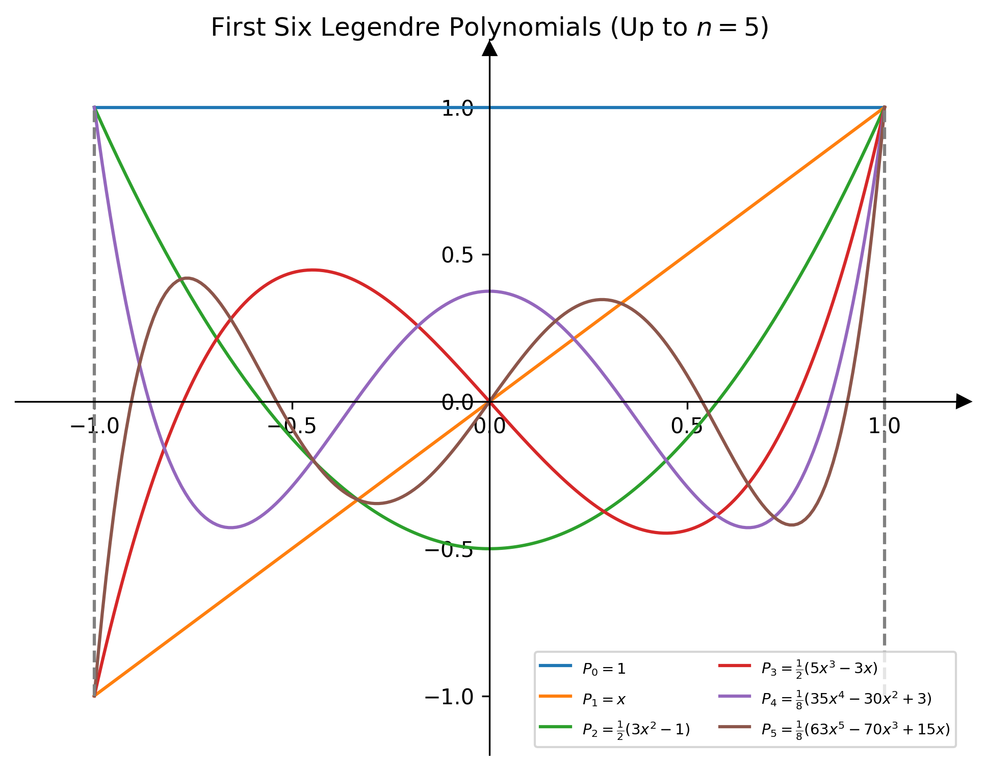
Now we take a look at a simple example: Express the polynomial \(p(x) = x^4 -3x^3 + 7x^2 + 4x -1 \) as a Legendre series. We begin by considering the Legendre polynomial of degree \(4\), \( P_4 = \frac{1}{8}(35x^4-30x^2+3) \). Comparing the leading term, we know that it must be \( p(x) = \frac{8}{35}P_4 + R_3 \) where \( R_3 = -3x^3 + (7-(-\frac{30}{35}))x^2 + 4x + (-1-\frac{3}{35}) = -3x^3 + \frac{55}{7}x^2 + 4x -\frac{38}{35} \) is the remainder polynomial of degree \( \leq 3\). Next, we have \( P_3 = \frac{1}{2}(5x^3 -3x)\) and \( R_3 = -\frac{6}{5}P_3 + R_2 \), with \(R_2 = \frac{55}{7}x^2 + (4-\frac{(3)3}{5})x -\frac{38}{35} = \frac{55}{7}x^2 + \frac{11}{5}x -\frac{38}{35} \). Then, it is not hard to see that \( R_2 = (\frac{55}{7})(\frac{2}{3})P_2 + R_1 = \frac{110}{21}P_2 + R_1 \) where \( R_1 = \frac{11}{5}x + (-\frac{38}{35}-(-\frac{55}{7(3)})) = \frac{11}{5}x +\frac{23}{15} \). Hence, the required Legendre series will be \( p(x) = \frac{8}{35}P_4 -\frac{6}{5}P_3 + \frac{110}{21}P_2 + \frac{11}{5}P_1 +\frac{23}{15}P_0 \).

Least-Square Approximation by Polynomials

If we are given a function \( f(x) \) and want to approximate it using a polynomial \(p_n(x)\) with a maximum degree of \(n\), then one of the natural choices is to take its Taylor series up to order \(n\). However, if our goal is to minimize the squared error, that is

\begin{align}
C[p] = \int_{-1}^1 [f(x) -p_n(x)]^2 dx \tag{2}
\end{align}

Then the desired polynomial will be the first \(n+1\) terms of the Legendre series of \( f(x) \), i.e. up to order \(n\):

\begin{align}
p(x) &= a_0P_0(x) + a_1P_1(x) + \cdots + a_nP_n(x) = \sum_{k=0}^n a_kP_k(x) \\
&= \sum_{k=0}^n \frac{2k+1}{2} (\int_{-1}^{1} P_k(x)f(x) dx) P_k(x) \tag{3}
\end{align}

The proof is as follows. By the last part, we know that all polynomials of degree \(n\) can be written as a Legendre series. Represent it as \( b_0P_0(x) + \cdots + b_nP_n(x) \), then the cost function (2) can be expressed as

\begin{align}
\int_{-1}^1 [f(x) -p_n(x)]^2 dx &= \int_{-1}^1 [f(x) -\sum_{k=0}^n b_kP_k(x)]^2 dx \\
&= \int_{-1}^1 f(x)^2 dx -\int_{-1}^1 2f(x) \sum_{k=0}^n b_kP_k(x) dx \\
&\quad + \int_{-1}^1 (\sum_{k=0}^n b_kP_k(x))^2 dx \\
&= \int_{-1}^1 f(x)^2 dx -2 \sum_{k=0}^n b_k \int_{-1}^1 f(x)P_k(x) dx \\
&\quad + \sum_{k=0}^n b_k^2 \frac{2}{2k+1} \\
&= \int_{-1}^1 f(x)^2 dx -2 \sum_{k=0}^nb_k \frac{2a_k}{2k+1} + \sum_{k=0}^n b_k^2 \frac{2}{2k+1} \\
&= \int_{-1}^1 f(x)^2 dx + \sum_{k=0}^n \frac{2}{2k+1} (b_k-a_k)^2 \\
&\quad -\sum_{k=0}^n \frac{2}{2k+1}a_k^2 \tag{4}
\end{align}

where we have recalled the orthonormalization properties of the Legendre polynomials, and completed the squares in the last line. Since \( f(x) \) and \( a_k \), hence the first and third summations are fixed, to minimize (4) means that we can only choose \( b_k = a_k \) so that the second summation of squares becomes zero and we are done.

Exercise

Find the first five terms of the Legendre series for \( \cos(\pi x) \).